Informacje o artykule
DOI: https://www.doi.org/10.15219/em106.1679
W wersji drukowanej czasopisma artykuł znajduje się na s. 71-78.
 Pobierz artykuł w wersji PDF
 Abstract in English
Jak cytować
Łabędzki, R. (2024). Decision making aided by Artificial Intelligence. e-mentor, 4(106), 71-78. https://doi.org/10.15219/em106.1679
E-mentor nr 4 (106) / 2024
Spis treści artykułu
- Abstract
- Introduction
- Utility
- Decision-making process
- Aid of Artificial Intelligence
- Summary
- References
Informacje o autorze
Decision making aided by Artificial Intelligence
Rafał Łabędzki
Abstract
The aim of the paper is to present how machine learning can support managers in the decision-making process. Analysis of the issue presented in this elaboration includes a review of the relevant literature on decision theory and utility as well as machine learning methods. The paper discusses possibilities of supporting managers through artificial intelligence in the context of stages of the decision-making process. It has been demonstrated that – thanks to artificial intelligence – it is possible to better estimate the expected utility of the alternatives that decision-maker choose from. Additionally, the paper presents an argument indicating that the use of machine learning makes the manager's decision-making process closer to the normative approach.
Keywords: decision-making process, artificial intelligence, utility, machine learning, management
Introduction
This paper presents the problem of using artificial intelligence by managers aid the decision-making process. The issue is of paramount importance as advancements in artificial intelligence have the potential to significantly reduce the gap between how decisions are made in practice and how they should be made according to the normative approach.
In this context, machine learning methods serve to link the normative approach to decision-making to the descriptive one. These methods provide managers with tools to better estimate the expected utility of the available alternatives by leveraging historical data and predictive models. The literature review performed in this paper focuses on combining decision theory with artificial intelligence with the aim to explore whether the aid of artificial intelligence can align human decision-making more closely with the normative model.
The first part of the paper discusses the use of utility as a criterion for comparing alternatives, which remains a cornerstone in both normative and descriptive decision-making frameworks. Following this, the text presents selected machine learning methods that can be employed to enhance decision-making processes. The final section outlines the role of artificial intelligence in these processes.
It is important to note that while this paper considers the application of artificial intelligence in decision-making from a local perspective, focusing on specific decision-making scenarios, the broader organizational implications of artificial intelligence integration, which are crucial for ensuring coherence and stability across an enterprise, are not addressed in this text. It should be kept in mind that a systemic approach to the adoption of artificial intelligence is essential for fully realizing its potential within an organization.
Utility
In order to study decision theory, it is well worth starting with a very interesting paradox, the so-called St. Petersburg Paradox. Its history dates back to 1713 when Nicholas Bernoulli began correspondence with Pierre Remond de Montmort. The subject of their letters was the "St. Petersburg Game", which involved repeatedly tossing a coin. Each game continues until the coin lands heads for the first time. The more tosses required to end the game, the larger the payout for the player. The amount of the payout is determined by the formula $2n, with n being the number of instances where the toss is heads. The expected payout can be described by the following formula (Peterson, 2023):

The paradox considered in the correspondence between the two distinguished mathematicians concerns the amount a player would be willing to pay for the opportunity to participate in the game. Since the expected value is theoretically infinite, would a participant pay any high amount for access? The scientists were unable to solve this puzzle for many years. It was not until 1728, when a Swiss mathematician Gabriel Cramer joined the correspondence, that a chance to find an answer emerged. Cramer proposed an innovative approach to perceiving the game's payout. According to his reasoning, a player would likely be guided by moral value rather than nominal value. In his calculations, he replaced monetary payouts with a value equal to their square root. Cramer justified his reasoning by arguing that a comparable earning for a poor person has much greater value than for a wealthy person. This approach meant that the initially infinite expected value of the game was limited to less than $3. Independently of Cramer, in 1732, Daniel Bernoulli, cousin of Nicholas Bernoulli, presented a similar line of reasoning but more comprehensive and based on a logarithmic function. He introduced the concept of utility and marginal utility, which became the basis of all subsequent research in decision theory (Bernoulli, 1954).
Utility – as a value used to compare the outcomes of possible decisions – has survived to this day. It became the basis of utilitarianism (Mill, 1844) and, consequently, the concept of homo economicus (Ingram, 1888). In the 20th century, thanks to von Neumann and Morgenstern (1947), Samuelson (1947), and especially Savage (1954), the concept of utility was used to create a mathematical apparatus describing rational decision-making by humans. This led to the development of the SEU (Subjective Expected Utility) theory. It is called normative because it describes how decision-makers should behave rather than how they actually do. In opposition to this approach, Simon (1955; 1957) proposed the theory of bounded rationality, taking into account the limitations of humans in decision-making. This is a descriptive theory. Simon's proposal did not reject the SEU model but was a more realistic interpretation of it. He maintained the existing understanding of utility but changed the method of its application and analysis when choosing the most advantageous decision. He primarily questioned the validity of building complete sets of alternatives and the real possibility for decision-makers to evaluate expected utility. It was not until Kahneman and Tversky (1979) that the perception of utility as a function of one's current endowment was abandoned in favor of viewing it as a function of changes in that endowment (prospect theory).
In this paper, normativity is understood as the pursuit of optimal decision-making, which aligns with the principles of the rational choice theory. This approach focuses on maximizing the expected utility of decisions, thereby enhancing the economic return for the decision-maker. The use of artificial intelligence in this context is intended to overcome the cognitive limitations of human decision-makers by providing a comprehensive analysis of the possible alternatives and their associated utilities, leading to decisions that adhere more closely to the normative ideal (von Neumann & Morgenstern, 1947). Importantly, this paper does not explore the ethical or social implications of decision-making aided by artificial intelligence. While utilitarianism – as developed by Bentham (1789) and Mill (1844) – emphasizes broader societal welfare, this study remains confined to the economic dimensions of decision-making. The exclusion of moral and ethical considerations allows for a focused examination of how artificial intelligence can improve decision accuracy from a purely economic standpoint, without the added complexity of evaluating public or customer welfare.
Decision-making process
Regardless of the approach, whether normative or descriptive, making a decision involves choosing one of the available alternatives for the decision-maker. Alternatives are actions that the decision-maker has to choose from. As a result of choosing one of the alternatives, the decision-maker expects certain future states to occur. Such states occur with a certain probability. Therefore, the decision-maker expects their occurrence but is not certain of it. Of course, the probability may be 100%, and then occurrence of the event is certain. However, it may happen that the chance of a given state occurring is not known. Then, the decision-maker makes a decision under the conditions of uncertainty, not risk, as is the case when the probability of an event occurring can be determined. According to utility theory, the decision-maker chooses a certain alternative to obtain a specified utility, which is a function of future states. Therefore, it can be said that the decision-maker only indirectly decides on the occurrence of a specific state because their real goal is to achieve the utility resulting from this state (Arrow, 1951). Decision-making, understood as choosing from among the available or permissible alternatives, is an element of a model consisting of the following components:
- Set of alternatives (A);
- Set of permissible (considered) alternatives (A` ⊂ A);
- Possible future states (S);
- Utility of future states (V(s), where s is an element of S);
- Information on which states will occur when choosing a given alternative;
- Information on the probability of states occurring when choosing a given alternative (Simon, 1955).
Set of alternatives (A)
The set of alternatives A encompasses all possible decisions that can be made. Making a decision is, in reality, choosing one of the alternatives, that is, one element from the set A (Simon, 1955). A single decision, or one of the alternatives, can lead to many possible future states, with the cumulative probability of these states occurring being equal to one (unless the decision is made under the conditions of uncertainty). This can be illustrated with the example of tossing a coin. If the decision-maker decides to toss a coin, they are choosing a 50% chance of the coin landing heads and a 50% chance that it will land tails. Thus, one element from the set of alternatives is assigned two possible future states; each with a certain probability. It should be noted that there is another future state associated with this choice: No result. Its probability is 0% in the case of the decision to toss a coin. However, if the decision-maker decides not to toss it, then the probability of the third state is 100%. This should not be forgotten, as the decision was about tossing or not tossing the coin.
Set of permissible (considered) alternatives (A` ⊂ A)
Sometimes the decision-maker only has a subset of the set of alternatives. This means that despite there being a larger number of possible choices, only a part of them is available to this particular decision-maker. These are permissible decisions, that is, those that meet additional limiting conditions, individual to the decision-maker (Simon, 1955). Such a situation can be simply illustrated by considering the purchase of milk in a grocery store. If the person making the decision, for example, is lactose intolerant, then from a potentially large set of alternatives, where each alternative represents the choice of a particular product, they can only choose those that do not contain lactose.
Possible future states (S)
The set S contains the possible future states that can occur with a certain probability depending on the alternative chosen by the decision-maker (Simon, 1955). It is important to note that the choice is merely the act of making a decision, and future states are events that occur as a result. In the decision-making model, each future state must result from a certain choice. Similarly, every choice must produce certain future events. Therefore, choices that do not lead to any of the events in the set S are not considered. Also, there are no elements of the set S, which are not the consequence of the decision to choose one of the alternatives from set A. The number of elements in set S is independent of the number of elements in set A. In an extreme case, it may be that all alternatives lead to one outcome. A situation where there is only one element in set A is not a decision-making situation, so such an extreme case does not occur.
Utility of future states (V(s), where s is an element of S)
The key to making a decision is determining the utility of future states. A given event – an element of set S – is merely an argument of the function determining its utility. Determining utility is very difficult. However, as Bernoulli and Cramer showed, it is utility, not nominal value, that determines the choices people make. Of course, the utility function is individual for each decision-maker, but universally it is characterized by diminishing marginal utility. This means that having more and more of a given good leads to progressively smaller increases in utility. Therefore, each decision-maker can obtain different utility values for each element of the same set S. It is easy to notice that this is the reason why people make different decisions in relatively similar decision-making situations. Utility does not have to be determined by any unit. In other words, the measure of utility does not have to be equivalents of currencies or energy or other units. To make a decision, only such value is needed that allows arranging the utility arising from the elements of set S from the highest to the lowest (Simon, 1955). This type of utility is referred to as ordinal utility. However, part of the scientific community associated with the decision theory is attempting to develop a measure of cardinal utility (Arrow, 1951).
Information on which states will occur when choosing a given alternative
Set A is connected to set S through information about which elements of set A can cause certain future states, that is, elements of set S (Simon, 1955). Both a one-to-one connection, where each alternative causes only one future state, and a situation where each alternative can cause many future states are permissible.
Information on the probability of states occurring when choosing a given alternative
Considering that the decision-maker makes choices under the conditions of risk, mere information about the connection between elements of set A and elements of set S is insufficient. It is necessary to know the probability of occurrence of the elements of set S given the choice of one of the alternatives from set A (Simon, 1955). Moreover, the elements of set S associated with a given alternative must exhaust all possible states induced by it. If each of the possible future states caused by a given alternative is assigned a certain probability of occurrence, then the sum of these probabilities must equal one. This ensures that the decision-maker is certain that one of the associated future states will occur as a result of their decision. In effect, the decision-maker has the possibility of determining the probability of utility arising from the occurrence of a given state. This means that for each of the alternatives, it is possible to calculate the expected utility value. Thus, the decision-maker can assess which alternative provides the greatest expected utility and make a choice.
Therefore, to make a decision, it is necessary to know the alternatives, determine what future states each of them can produce and with what probability, estimate the utility resulting fromoccurance of the future states, and finally choose the alternative that results in the highest expected utility. To make this possible, work needs to be done involving:
- Gathering alternatives.
- Determining future states and the probability of their occurrence depending on the occurrence of each alternative.
- Assessing the utility of each state.
Each of these tasks can be extremely time-consuming. Sometimes, it may turn out that gathering only a limited number of alternatives is more reasonable; as considering all the possible ones would be unprofitable or impossible. Reaching a decision based on a detailed analysis of all the possible alternatives and their resulting expected utilities is making an optimal choice. Such an approach is characteristic of the normative approach. However, if the decision-maker has only a limited number of considered alternatives, they can still make a satisfactory (good enough) choice, as long as the alternatives are permissible. The discussion between the proponents of the normative and descriptive approaches is concerned with, among other things, whether people make optimal or good enough choices. Simon, who proposes the concept of bounded rationality, advocates that people do not consider all the possible alternatives but only a certain limited number of those. Moreover, estimating the probability of occurrence of each future state is also very difficult and questioned by Simon. Finally, estimating the utility of each element of set S seems to be an almost impossible task. Thus, the discrepancy between how people should, from a rational point of view, make decisions, and how they actually make them, is very large. It mainly arises from the capabilities that humans have (Holska, 2016). Therefore, one may ask whether, if humans had the support of artificial intelligence, their decision-making could get closer to the approach advocated in the normative stream?
To fully answer such a question, it is necessary to consider how artificial intelligence could aid humans in each of the three tasks mentioned earlier. In this paper, only one of them will be considered – determining the probability of occurrence of future states. This is a significant simplification, but it seems justified as it allows for a clear definition of the role of artificial intelligence as an entity aiding the manager. It should also be noted that an additional limitation has been applied in the form of describing the possibilities of aiding the decision-maker by artificial intelligence only in business decisions, for which the decision-maker has historical data that allow the use of machine learning for classification of or predicting the values related to the future events.
Aid of Artificial Intelligence
Artificial Intelligence
Artificial Intelligence is a field of science involved in creating computer models that simulate aspects of human thinking (Newell & Simon, 1976). One of the important branches of artificial intelligence is machine learning, which allows computers to autonomously create solutions to problems based on data (Goodfellow et al., 2016; Turing, 1950).
Having data may, but does not necessarily, enable the application of artificial intelligence. Not all data are suitable for use in machine learning. However, if a manager has data of sufficient quality, they can use artificial intelligence to answer at least two questions. The first one is: "What can be said about what there is?". The second question is: "What can be said about what there will be, based on what there is, using knowledge of what there was?".
The answer to the first question is provided by a branch of machine learning called unsupervised learning. As a result of using methods of this kind, it is possible, for example, to group the objects in the data into clusters. Such knowledge can be useful for various analyses that managers conduct (Natingga, 2018).
The second question is answered by a branch of machine learning known as supervised learning. Supervision in this group of methods means that historical data used to train artificial intelligence models contain both: 1) the parameters of the decision-making situation, which were considered when making decisions in the past, and 2) the outcome of those decisions in the form of occurrence of some states, that is, elements of set S (Boschetti & Massaron, 2015). Knowledge of which sets of parameters caused certain states in the past allows supervised machine learning to answer the question of what states might occur in the future and with what probability, depending on the parameters of the current decision-making situation. For this reason, this chapter will discuss supervised machine learning methods and their application to predicting the probability of occurrence of states from set S.
Data
Supervised machine learning is based on historical data. Since the data contain both the parameters of past decisions (further referred to as arguments collected in matrix X) and the effects of these decisions in the form of events from set S (further referred to as values collected in vector Y), it is possible to examine their interrelations and establish rules determining that for certain elements of set X, specific elements of set will Y occur (Boschetti & Massaron, 2015).
Among those working with artificial intelligence, the saying "garbage in, garbage out" is popular. If low-quality data are used to create an artificial intelligence model, then as a result, the prediction generated by such a model will be of low quality. Therefore, it is clear that high-quality data are necessary to train a high-quality model. This means, among other things, that the data within a given set must be comparable (contain the same parameters), must be relevant from the point of view of the consequences of the decisions made, and there must be enough of them. Depending on whether artificial intelligence is used for classification or for regression, the data forming vector Y must be of an appropriate type (Boschetti & Massaron, 2015).
Machine learning models
The key concept that needs defining is a machine learning model. It can be thought of as a mathematical function that transforms input data into a prediction (Murphy, 2021). Although this is a significant generalization, it reflects reality. Machine learning is a process in which a model is created. The job of a person creating it involves selecting the appropriate type of model and then training it using data. The result should be satisfying model parameters.
There are many types of machine learning models. It is worth noting that the use of a particular model should depend on the relevant needs (Boschetti & Massaron, 2015). In the case of models that can support estimation of the probability of future events – that is, elements of set S – it seems reasonable to consider those models that enable classification. Classification involves assigning a given object to one of the predefined classes with a certain probability. For example, based on information about a customer, they can be assigned to a specific class.
Logistic regression. One of the machine learning methods that can be used for classification is logistic regression. This method allows for binary classification. Its application can result in assigning a given object to one of two classes (Natingga, 2018). If making a decision requires classification of objects into more than two groups, another type of machine learning model should be used.
It's important to note an additional benefit of using logistic regression. Among the three machine learning methods presented in this paper, logistic regression is one of the two that have interpretable parameters. This means that the trained not only classifies observations, but also provides information which of the model's parameters have the greatest significance for the predictions being created. This information is valuable both for the person developing the model and for those responsible for data collection (Natingga, 2018).
Decision tree. A decision tree is a machine learning method that, even judging by its name, seems destined for use in solving decision problems. The decision tree is a very good machine learning method that allows for classifying an object into more than two classes and even predicting values (Natingga, 2018).
Like logistic regression, a decision tree has interpretable parameters. Decision trees have a tree like structure where each node represents a decision criterion and each edge represents the outcome of that decision. The leaves of the tree represent class labels or predicted values. The tree structure is understandable even to those without advanced statistical knowledge, which is a very important advantage of this method. As far as algorithms creating decision trees are concerned, the quality of the split is assessed based on various measures, such as information gain, for example. A decision tree makes a split according to decreasing information gain. This means that by reading a decision tree from the top, that is, from the first node, one can quickly determine which of the examined parameters are more important and which are less important from the point of view of the split (Raschka & Mirjalili, 2019).
Perceptron and neural network. Many people undoubtedly associate artificial intelligence with neural networks. A neural network is a model of artificial intelligence that, in principle, is designed to reflect the functioning of the human brain. A neural network is composed of many perceptrons. Each perceptron is a reflection of a neuron in the human brain. Perceptrons are interconnected and that way they form a neural network. Like other machine learning models, a neural network, based on input data, provides predictions both in the form of classification and specific values. A neural network can classify objects into many classes and provides information about the probability of assigning a given object to each of them (Raschka & Mirjalili, 2019).
A neural network can be used for decision-making in a similar way as the decision tree or logistic regression. Unlike them, the reasons why a neural network assigns specific objects to classes are very difficult or impossible to ascertain. Using a neural network leads only to solving the problem of predicting probability. In this case, the decision-maker or the person developing the machine learning model does not have the possibility to know the weights of specific parameters, which is not the case with the other two methods described.
It's important to note that a neural network is not inherently a better classifier than a decision tree or logistic regression. Choosing the best classifier is only possible in the context of a specific problem.
Model training
The goal of model training is to achieve satisfying parameters. In the case of models whose task is classification, the aim of training is to achieve the best possible quality of this classification. In other words, the task of the creator of a model is to select its parameters so that the model will determine the probability of assigning a given object to one of the predefined classes as accurately as possible (Raschka & Mirjalili, 2019).
Training an artificial intelligence model is a non-trivial task. As mentioned earlier, the quality of this model depends on the quality of the data available for its training. However, even assuming that there is high-quality data available, attention should be paid to the so-called phenomenon of overtraining the model and the related issue of generalization. It may turn out that a model highly rated based on historical data makes worse predictions based on new data than a seemingly weaker model. The person working on training the model should take into account a series of important parameters that determine the value of this model for managers making decisions aided by it (Raschka & Mirjalili, 2019).
Using the model in decision making
According to DMN (i.e., Decision Model and Notation), an artificial intelligence model can be placed in a decision-making model as a source of knowledge aiding decision-making logic. The prediction provided by the model is used to choose an alternative based on the logic described in a decision table (Object Management Group, 2023).
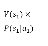
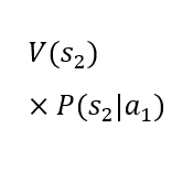
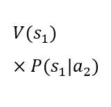
Let an example of application of the model be a decision-making situation concerning granting a loan. To create a machine learning model in such a case, historical data are needed that contain information about two types of clients – those who repay and those who do not repay loans. The data must include both parameters characterizing the clients – matrix X – and a label assigning the client to one of the classes – vector Y. The decision-maker is the person granting the loan. The available alternatives are: 1) granting a loan and 2) not granting a loan. Possible future situations are: 1) timely repayment, 2) non-repayment, and 3) rejection of the client. The decision-making situation is illustrated by the following table.
Table 1
Decision to grant a loan
| States (S) | ||||
| Alternatives (A) | Expected utility of the alternative | Timely repayment (s1) | Non-repayment (s2) | Rejection of the client (s3) |
| Granting a loan (a1) | 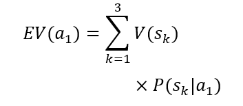 |
 |
 |
 |
| Not granting a loan (a2) |  |
 |
 |
 |
Source: author's own work.
The rows of the table present two alternative choices. Each alternative is characterized by an expected utility. The decision-maker should choose the alternative with the higher expected utility. It is assumed that the utility of states V(sk) is established. The dynamic value in the table is the probability of occurrence of the future states given the choice of a particular alternative P(sk|ai). In the case under consideration, the probability of the third state occurring is 0% for the first alternative and 100% for the second alternative. The probability of the first and second states occurring in the case of the second alternative is 0%. However, the probability of the first and second states occurring in the case of the first alternative is not known. The artificial intelligence model can be used to determine these probabilities. Thanks to its predictions, it is possible to calculate the expected utility of the first alternative and compare it with the expected utility of the second alternative, which is constant, as it depends only on the utility of the state in which the client is rejected. As can be easily seen, a loan will only be granted in the situation where the probability of the first state occurring under the first alternative is high enough for the expected utility of the first alternative to be higher than the expected utility of the second alternative. Considering the constant values mentioned above, it is possible to determine such a level of probability of the first state occurring under the first alternative for which it will be known that it conditions the decision to grant a loan. Such a threshold value can be used to construct a decision table for which the source of knowledge will be the machine learning model.
If granting a loan requires:

and it is known that:
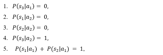
then:
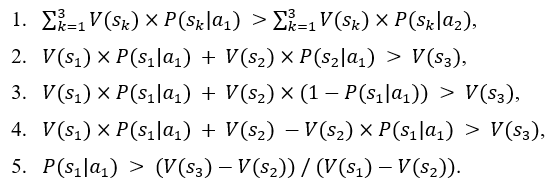
Therefore, there is a predefined probability level of the first state occurring under the first alternative, and if exceeded, it will prompt the choice of this particular alternative. In this specific case, it can be seen that this value is determined by the ratio of the excess of the utility of the third state over the second to the excess of the utility of the first state over the second. It is easy to see that for the decision-maker to be able to conduct business related to granting loans at all, the utility of the first state (i.e., of granting a loan) must be greater than the utility of the third state. The greater the excess of the utility of granting a loan over the state of inactivity (i.e., of the third state), the lower the threshold values for the probability of the first situation occurring under the first alternative are needed. Below is a decision table built based on the determined threshold value of the probability of the first situation occurring when deciding to grant a loan.
Table 2
Decision table
| Input: P(s1|a1) | Output |
|
Possible inputs: > (V(s3) - V(s2)) / (V(s1) - V(s2)), <= (V(s3) - V(s2)) / (V(s1) - V(s2)) |
Possible outputs: Granting a loan, Not granting a loan |
| > (V(s3) - V(s2)) / (V(s1) - V(s2)) | Granting a loan |
| <= (V(s3) - V(s2)) / (V(s1) - V(s2)) | Not granting a loan |
Source: author's own work based on Decision Model and Notation, Object Management Group, 2023 (https://www.omg.org/spec/DMN/1.5/Beta1/PDF)
The decision table can be an element of decision-making logic within a decision model described according to DMN. The source of knowledge for this decision table is the artificial intelligence model, which, based on customer parameters, returns the probability of the first state occurring in the case of a decision to grant a loan.
In order to develop a decision table that cooperates with a artificial intelligence model and to use it, collaboration between humans and machines is required. Division of responsibilities within this collaboration would be as follows:
- The human is responsible for defining the set A, that is, the available or permissible alternatives;
- The human is responsible for defining the possible future states S;
- The human is responsible for assigning utility V(s) to each of the states;
- The human is responsible for defining the probability intervals for the occurrence of states from set S, which, if exceeded, trigger changes in the order of the expected utility of alternatives A.
- Artificial intelligence is responsible for providing a prediction of the probability of states (S) occurring depending on the parameters of a given decision-making situation.
As a result of such a collaboration, a manager making decisions can base them on a larger number of parameters defining the decision-making situation and better predict the expected utility than a manager without the support of artificial intelligence.
Summary
This paper considered only one of the tasks related to decision-making in the context of the possibilities of aiding decision-makers with artificial intelligence. Of course, it is worth answering the question of how artificial intelligence can aid managers in gathering alternatives and estimating utility. However, just showing how a computer can help decision-makers determine the probability of future events occurring allows us to state that with the use of artificial intelligence a manager can reduce their limitations and bring their decision-making process closer to the model proposed in the normative approach.
The example considered above (regarding a decision to grant a loan) is primarily concerned with a situation where the client initiates contact with the decision-maker. However, artificial intelligence has the potential to enhance decision-making further by proactively identifying potential clients who should be approached. Through predictive analytics, artificial intelligence can analyze vast amounts of customer data to segment and select high-value prospects, allowing organizations to take a more strategic, forward-looking approach. This proactive capability shifts the role of artificial intelligence from merely assessing those who approach the decision-maker to actively identifying and engaging potentially valuable clients before they express a need to do so.
References
- Arrow, K. J. (1951). Alternative approaches to the theory of choice in risk-taking situations. Econometrica, 19(4), 404-437. https://doi.org/10.2307/1907465
- Bentham, J. (1789). An introduction to the principles of morals and legislation. T. Payne and Son.
- Bernoulli, D. (1954). Exposition of a New Theory on the Measurement of Risk. Econometrica, 22(1), 23-36. https://doi.org/10.2307/1909829
- Boschetti, A., & Massaron, L. (2015). Python data science essentials. Packt Publishing Ltd. Goodfellow, I., Bengio, Y., & Courville, A. (2016). Deep learning. The MIT Press, 19, 305-307. https://doi.org/10.1007/s10710-017-9314-z
- Holska, A. (2016). Teorie podejmowania decyzji. In K. Klincewicz (Ed.), Zarządzanie, organizacje, organizowanie przegląd perspektyw teoretycznych (pp. 239-251). Wydawnictwo Naukowe Wydziału Zarządzania Uniwersytetu Warszawskiego. https://timo.wz.uw.edu.pl/wp-content/uploads/2016/09/Klincewicz-Krzysztof-red-Zarzadzanie-organizacje-i-organizowanie.pdf
- Ingram, J. K. (1888). A history of political economy. The Macmillan Company.
- Kahneman, D., & Tversky, A. (1979). Prospect theory: An analysis of decision under risk. Econometrica, 47(2), 263-292. https://doi.org/10.2307/1914185
- Mill, J. S. (1844). Essays on some unsettled questions of political economy. John W. Parker.
- Murphy, K. P. (2021). Probabilistic Machine Learning: An introduction. MIT Press.
- Natingga, D. (2018). Data Science Algorithms in a Week: Top 7 algorithms for scientific computing, data analysis, and machine learning. Packt Publishing Ltd.
- Newell, A., & Simon, H. A. (1976). Computer science as empirical inquiry: symbols and search. Communications of the ACM, 19(3), 113-126. https://doi.org/10.1145/360018.360022
- Object Management Group. (2023). Decision Model and Notation. https://www.omg.org/spec/DMN/1.5/Beta1/PDF
- Peterson, M. (2023). The St. Petersburg Paradox. The Stanford Encyclopedia of Philosophy. https://plato.stanford.edu/archives/fall2023/entries/paradox-stpetersburg
- Raschka, S., & Mirjalili, V. (2019). Python machine learning: Machine learning and deep learning with Python, scikit-learn, and TensorFlow 2 (3rd ed.). Packt Publishing Ltd.
- Samuelson, P. A. (1947). Foundations of economic analysis. Harvard University Press.
- Savage, L. J. (1954). The foundations of statistics. John Wiley & Sons.
- Simon, H. A. (1955). A behavioral model of rational choice. Quarterly Journal of Economics, 69(1), 99-118. https://doi.org/10.2307/1884852
- Simon, H. A. (1957). Models of man; social and rational. Wiley.
- Turing, A. M. (1950). Computing machinery and intelligence. Mind, 59(236), 433-466. https://doi.org/10.1093/mind/LIX.236.433
- Von Neumann, J., & Morgenstern, O. (1947). Theory of games and economic behavior (2nd rev. ed.). Princeton University Press.


 https://orcid.org/0000-0002-0239-4125